To create a school receipt template in Google Sheets, start by setting up a simple table with clear columns for the necessary information. Use columns for the student’s name, date, item description, quantity, price, and total cost. This setup helps keep everything organized and easy to read.
Next, apply basic formulas to automatically calculate totals. For example, use the formula =B2*C2 to multiply the quantity and price for each item. This reduces manual entry errors and saves time. You can then sum up all the totals at the bottom using =SUM(D2:D10), where D is the total cost column.
For a more professional look, format the template with borders around each cell and shade the header row to make it stand out. Add a school logo or any other custom details you might need. You can also create a dropdown menu for selecting different items or categories using Data Validation to further streamline the process.
Detailed Guide for Creating a School Receipt Template in Google Sheets
Creating a school receipt template in Google Sheets is a simple task that can help track payments, donations, and fees. Follow these steps to design a functional template that suits your needs.
1. Set Up the Basic Structure
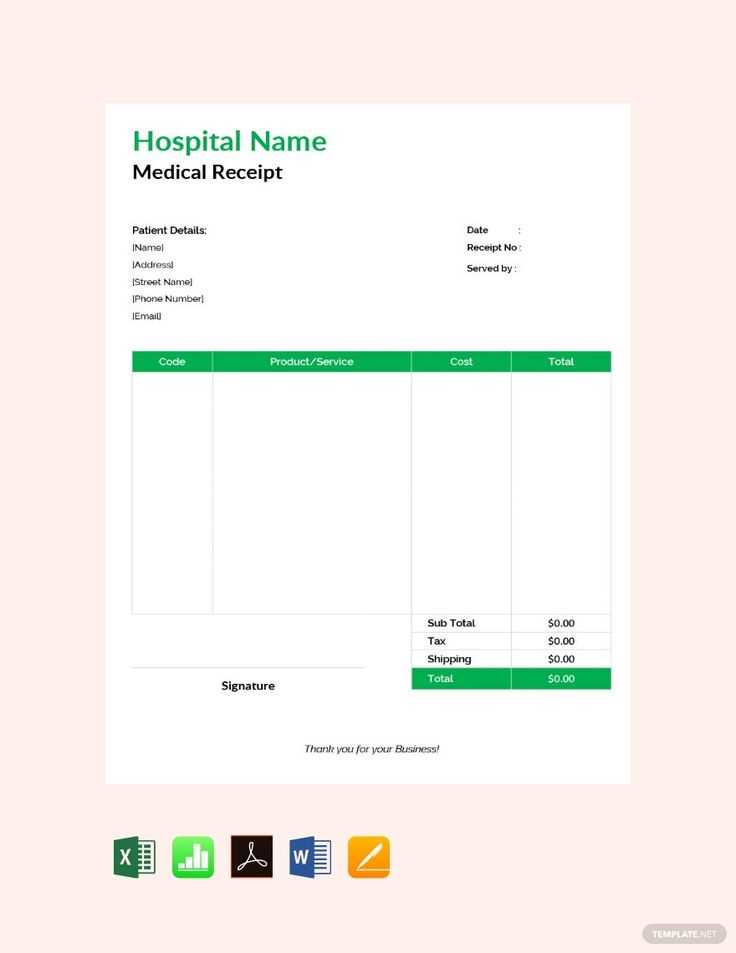
Start by opening a new Google Sheets document. Label the first few columns for the necessary receipt details:
- Date – The date of the transaction.
- Receipt Number – Assign a unique number for tracking purposes.
- Student Name – Name of the student making the payment.
- Amount – The payment amount.
- Description – A brief description of what the payment is for (e.g., tuition, materials).
These columns will form the backbone of your template, keeping the information organized and easy to read.
2. Apply Formatting and Functions
Now, adjust the columns for better presentation:
- Merge Cells for the header row (Date, Receipt Number, etc.), making the labels more prominent.
- Format Columns to match the type of data. For example, set the “Amount” column to currency format.
- Conditional Formatting can be applied to highlight overdue payments or specific categories, like tuition or fees.
Additionally, you can use basic functions like SUM at the bottom of the “Amount” column to calculate the total amount collected.
3. Add Customization Features
- Drop-Down Lists: Use data validation to create drop-down lists for fields like “Payment Method” (Cash, Check, Credit Card).
- Timestamp: Insert a timestamp function to record the exact time when the receipt was created.
- Automated Receipt Numbering: Use a simple formula like
=ROW()-1to automatically generate receipt numbers as new rows are added.
These customization features will streamline the data entry process and make the template more adaptable to your specific needs.
4. Save and Share
Once the template is set up, save the document for future use. You can also share it with other school staff for easy access and collaboration by clicking the “Share” button in Google Sheets.
Setting Up the Basic Structure for a School Receipt Template
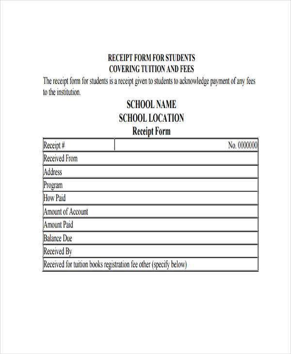
Begin by creating a clean and organized layout. Use Google Sheets to set up a simple grid with clearly defined rows and columns for each element of the receipt. Divide the grid into sections: school details, student information, payment breakdown, and total amount. This structure keeps the data easy to input and read.
Start with labeling the first few columns for essential information: “Date,” “Receipt Number,” and “Payment Method.” These fields will remain consistent across all receipts. In the subsequent columns, include the student’s name, grade, and ID number for easy reference. Make sure to leave enough space to accommodate different data lengths without cluttering the sheet.
Next, add a column for the “Description of Service,” where details about the fee being paid, such as tuition, extracurriculars, or materials, can be listed. Each service or charge should be in a separate row for clarity. The “Amount” column will follow next, where you’ll input the cost of each service. A final column for the “Total” will sum the amounts and give a clear final value for the receipt.
Finally, consider adding simple formulas to automatically calculate totals. For example, use the SUM function to add up all amounts in the “Amount” column. This saves time and reduces errors. Keep the format consistent, and adjust column widths as needed to prevent text from spilling over into other areas.
Customizing Columns for Different Payment Types and Discounts
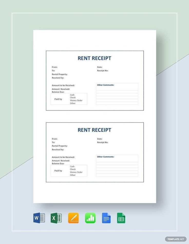
To tailor your Google Sheets receipt template for various payment methods, create separate columns for each payment type, such as “Cash,” “Credit Card,” and “Bank Transfer.” This allows clear tracking of individual payments and ensures that the receipt reflects the exact amounts processed through each method.
For payment types that offer discounts, add columns like “Discount Applied” and “Final Amount.” Use formulas to calculate the discounted total by applying the discount percentage to the original price. You can also add conditional formatting to highlight cells where discounts are applied, making it easier to track reductions.
Incorporate drop-down menus for each payment method and discount type using data validation. This ensures that the entries remain consistent and minimizes errors. For instance, under the “Payment Method” column, users can select from a predefined list of options, which simplifies data entry and keeps everything organized.
Additionally, for invoices with multiple discounts, add a “Discount Reason” column to track the type of discount applied (e.g., “Seasonal Offer,” “Bulk Purchase,” or “Loyalty Discount”). This adds transparency and makes it easier to assess which discounts are most frequently used, improving future decision-making.
Using Formulas to Automate Total Calculations and Taxes
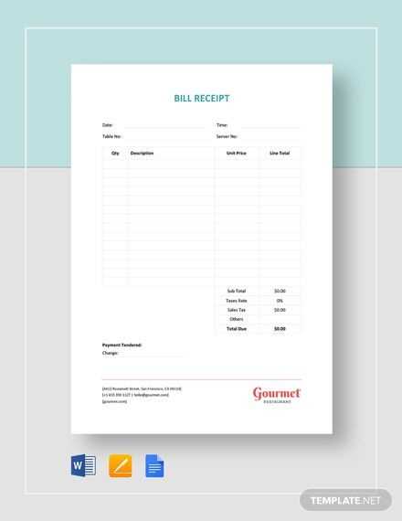
To simplify the process of calculating totals and taxes in your Google Sheets school receipt template, use formulas that automate these tasks. Start with basic arithmetic functions like SUM to total amounts. For example, in a cell, you can enter the formula:
=SUM(B2:B10)
This will add all values in the range from B2 to B10. Adjust the range as needed depending on your data. Next, to calculate taxes automatically, use a multiplication formula. For instance, if you want to apply a 5% tax to the total amount, use:
=SUM(B2:B10)*0.05
This will calculate 5% of the total sum in the range. You can place this formula in the cell where you want to show the tax amount. To display the grand total (subtotal plus tax), combine both formulas:
=SUM(B2:B10)+(SUM(B2:B10)*0.05)
This formula adds the subtotal and the calculated tax. You can update the tax rate as needed by changing the percentage in the formula.
Automating Discount Calculations
If you offer discounts, you can add another layer of automation by calculating them directly in your sheet. For example, if a 10% discount applies, use this formula:
=SUM(B2:B10)-(SUM(B2:B10)*0.10)
This subtracts 10% from the subtotal automatically. Combine this with tax calculations for a final total:
=((SUM(B2:B10)-(SUM(B2:B10)*0.10))+(SUM(B2:B10)-(SUM(B2:B10)*0.10))*0.05)
Using Conditional Logic for Dynamic Pricing
For further flexibility, apply conditional logic with the IF formula. This allows you to calculate different tax rates based on the total amount. For example, if the total exceeds $100, apply a 10% tax; otherwise, apply 5%. Use this formula:
=IF(SUM(B2:B10)>100, SUM(B2:B10)*0.10, SUM(B2:B10)*0.05)
This checks whether the total is greater than $100 and applies the corresponding tax rate accordingly. Using these formulas will keep calculations precise and reduce manual errors.
