Creating a credit card receipt template in Excel is a simple yet powerful way to track your transactions and maintain clear records. Whether you are a small business owner or managing personal expenses, having a template ready can save you time and help you stay organized.
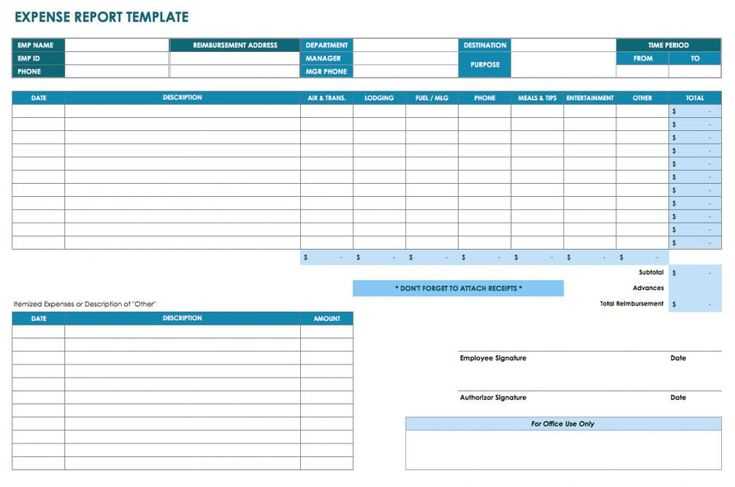
Start by customizing your template to include fields like transaction date, merchant details, purchase amount, and payment method. These details ensure accurate tracking of all charges, making it easy to cross-reference against your credit card statements.
Additionally, consider using Excel’s built-in formulas to automatically calculate totals and apply taxes where necessary. This feature enhances the template’s utility by reducing manual input and preventing errors in calculations.
By keeping everything in a single, organized sheet, you can quickly generate reports or summaries of your credit card activity, simplifying both personal budgeting and financial auditing. Make sure to update the template regularly for maximum accuracy and consistency.
Credit Card Receipt Template Excel: A Practical Guide
Creating a credit card receipt template in Excel can simplify tracking transactions and ensure accurate record-keeping. Start by setting up a clear, structured table to capture key details of each transaction. Include columns for the date, merchant name, transaction amount, credit card number (masked for privacy), and any applicable taxes or discounts.
Use Excel’s built-in features to make the template more functional. Conditional formatting can highlight large transactions or overdue payments. You can set up formulas to automatically calculate totals or tax amounts, reducing manual entry errors. Additionally, create a drop-down list for common merchants or payment types to speed up data entry.
For easier tracking, add a column for payment status (paid or pending). This will help you stay organized and reduce the chances of missed payments or discrepancies. Make sure to protect the template with password encryption if you’re handling sensitive credit card information.
Lastly, consider creating a simple summary sheet that pulls data from your transaction logs. This way, you can generate reports with ease, tracking total spending or categorizing expenses without manually compiling numbers. A well-organized Excel template will save time and provide clarity on your credit card transactions.
How to Create a Custom Credit Card Receipt Template in Excel
To create a custom credit card receipt template in Excel, follow these steps to design a structured and easy-to-use format tailored to your needs.
Step 1: Set Up the Basic Structure

- Open a new Excel workbook.
- Adjust the column widths to fit key information such as transaction details, amounts, and dates.
- Create headers for each section, such as “Date,” “Merchant Name,” “Transaction Amount,” “Payment Method,” and “Approval Code.” This will help organize the data clearly.
Step 2: Format Cells for Specific Data Types

- Format the “Date” column to display the correct date format (e.g., MM/DD/YYYY).
- Use currency formatting for the “Transaction Amount” column to display the correct amount in your preferred currency.
- Ensure other columns, like “Merchant Name” and “Approval Code,” are set to “General” or “Text” format to avoid formatting issues.
Step 3: Add Conditional Formatting for Easy Reading
- Use conditional formatting to highlight transactions based on specific criteria, such as amounts over a certain value or expired dates.
- Apply different colors to the rows to differentiate between successful and unsuccessful transactions.
Step 4: Include Formulas for Calculation (Optional)
- If you want to calculate totals or perform any other operations, use formulas. For example, use the SUM formula to calculate the total transaction amount in the “Transaction Amount” column.
- Use IF statements to categorize transactions into specific types (e.g., successful, pending, or failed).
Step 5: Add Company Branding (Optional)

- Incorporate your company logo or color scheme to make the receipt look professional and consistent with your brand.
- Adjust the font size and style for headers and other important information to ensure clarity and readability.
Step 6: Save and Reuse the Template
- Once you’re satisfied with the layout, save your template as an Excel file (.xlsx) or as a template file (.xltx) so you can reuse it for future transactions.
How to Add Payment Details and Taxes to Your Credit Card Receipt Template
To add payment details and taxes to your credit card receipt template, first make sure you have clear sections for each element. Start by including the total amount charged, showing the original price before taxes, the tax amount, and the final amount after taxes.
In your template, create a row or column for “Payment Method” where you will specify the card type (e.g., Visa, MasterCard) and the last four digits of the card number. This ensures clarity for both the customer and your records.
Next, calculate the tax by applying the appropriate tax rate to the pre-tax amount. Include a label such as “Tax” next to the calculated figure for easy identification. If you are dealing with multiple types of taxes (e.g., federal and state), list each separately with their respective amounts.
Ensure the total reflects the sum of the price and all applicable taxes. This total should be clearly labeled, for example, as “Total Amount Charged.” Double-check for accuracy before saving or printing the receipt.
Additionally, it is helpful to add a payment reference or transaction ID number for tracking purposes. This provides a direct link to the payment record in your system for future reference.
How to Automate the Calculation of Total Amount Using Excel Functions
To calculate the total amount automatically, use the SUM function in Excel. Place your item prices in a column (e.g., column B). In a new cell, type the formula: =SUM(B2:B10), assuming your values are in cells B2 to B10. This will sum all the values in that range.
If you have additional columns for quantity (e.g., column C) and need to calculate the total amount for each item, multiply the price by the quantity. Use this formula in a new column (e.g., column D): =B2*C2. Copy this formula down for all rows with data.
For a grand total, you can sum all the individual totals in column D with another SUM function: =SUM(D2:D10).
If you want to automatically include or exclude items based on specific conditions (e.g., only sum totals for items above a certain price), use the SUMIF function. For example, to sum the totals for all items priced over $50, the formula would be: =SUMIF(B2:B10, “>50”).
To calculate taxes or discounts, apply the appropriate formula based on the tax rate or discount percentage. For example, for a 10% tax, use: =D2*0.1 to find the tax for an individual item, or sum it up for all items with =SUM(D2:D10)*0.1.