A well-organized Receipts and Payments Excel template is the simplest way to track all your financial transactions. It lets you record income and expenses easily, making it effortless to stay on top of your finances. With a clear structure, this tool ensures that you never miss important details.
Customize your template to suit your needs. Whether you are running a small business or managing personal expenses, an Excel sheet provides the flexibility to adapt categories, set up automatic calculations, and create summaries. This way, you can focus more on making decisions and less on manual tracking.
Regular updates to your records are key. Make it a habit to enter receipts and payments as soon as they occur. This ensures that your data remains accurate, and you can immediately spot any discrepancies or patterns that may require attention. A consistent approach is the foundation of smooth financial management.
Here are the corrected lines without word repetitions:
Ensure each category is clearly separated in your Excel sheet, such as “Receipts” and “Payments”, to keep track of each transaction accurately.
Label each column with concise headers like “Date”, “Description”, “Amount”, and “Balance”. This helps avoid confusion while reviewing the entries.
Recommendations for Entries
For receipts, list the payment sources separately from any expenses, detailing each transaction date and amount received.
For payments, break down costs into individual line items, which can be categorized by type (e.g., utilities, salary, office supplies).
Adjusting Totals
Use formulas like SUM to automatically calculate totals in separate columns for better accuracy. This ensures no overlap in calculations between receipts and payments.
By maintaining a clear structure, the template will provide an organized view of your financial transactions, allowing for easy tracking and analysis.
- Receipts and Payments Excel Template
Start by customizing a receipts and payments template to track financial transactions. Use Excel’s built-in features like drop-down lists for categories, so entries stay organized. Create separate columns for date, description, payment type, amount, and balance to easily track income and expenses.
Linking formulas can automate calculations. For example, use SUM to calculate totals for both receipts and payments. This reduces errors and ensures that the balance is always up-to-date. You can also incorporate conditional formatting to highlight overdue payments or high amounts.
To make it easier to identify trends, sort your data by date or category. Excel’s pivot table functionality helps summarize large amounts of data, giving you quick insights into your financial performance.
Consider using templates from trusted sources as a starting point, but tailor it to your needs by adding columns for additional information such as payment method or invoice numbers. Regularly update the template to reflect new transactions for accuracy.
To create a functional receipt and payment form in Excel, first open a new spreadsheet. Begin by labeling the columns: Date, Description, Receipt Amount, Payment Amount, and Balance. These fields will allow you to track both incoming and outgoing transactions efficiently.
Step 1: Define Your Columns
Set up the columns with the following headers:
- Date: The date of the transaction.
- Description: A brief note about the transaction.
- Receipt Amount: Enter the money received here.
- Payment Amount: Enter the money paid out in this column.
- Balance: This column will calculate the running balance after each transaction.
Step 2: Add Formulas

In the Balance column, enter a simple formula to track the changes in the balance. In the first row of Balance (let’s assume row 2), enter the formula:
=C2-D2
. This will subtract the Payment Amount from the Receipt Amount. For subsequent rows, the Balance formula should be adjusted to account for the previous balance:
=E2+C3-D3. This will ensure the running balance is updated correctly after every transaction.
Save the template and make sure to adjust the cell references when you expand the table for more transactions.
To tailor the Excel template to your needs, start by adjusting the column headers. Select the column you want to modify, then right-click and choose “Insert” to add new columns. You can rename the columns to better reflect the type of data you’re working with, such as “Payment Method” or “Receipt Number.” This allows you to track specific information clearly and consistently.
Next, use data validation to limit the types of entries for each column. For example, in the “Payment Method” column, you can create a drop-down list with options like “Cash,” “Credit Card,” and “Bank Transfer.” This ensures uniformity in the data input, reducing errors and simplifying analysis.
To further refine the columns, consider using conditional formatting. Highlight columns based on criteria, such as payments above a certain amount or overdue receipts. This visual cue makes it easier to spot critical information quickly.
Finally, don’t forget to adjust column widths to fit the content properly. Double-click the boundary between columns to auto-resize, or manually drag to make sure all your entries are fully visible. Customizing your columns in this way helps you maintain a well-organized and easy-to-read template.
To automatically calculate total income and expenses in an Excel template, leverage built-in functions like SUM and SUMIF. These functions simplify the process of summing up data in different categories without manual calculations.
Set Up Categories
- Organize your data into distinct categories: income, expenses, and specific subcategories (e.g., salary, bills, groceries).
- Use separate columns for each category to ensure clarity and easy data entry.
Implement SUM Function
- In the income and expense columns, use the SUM function to calculate the totals. For example, type
=SUM(A2:A10)to add up all values in cells A2 to A10. - To calculate total expenses, apply the same function to the relevant column:
=SUM(B2:B10).
Use SUMIF for Conditional Calculations

- To calculate income or expenses based on specific criteria, use SUMIF. For example, if you want to calculate income from a particular source, use
=SUMIF(A2:A10, "Salary", B2:B10), where “Salary” is the condition, and B2:B10 contains the amounts. - This can be helpful for tracking specific expense categories, like utilities or entertainment.
These simple Excel functions automate calculations, saving time and reducing the chance for errors. Keep your data organized, and Excel will handle the totals for you.
Set up a clear system for tracking receivables and liabilities. In your Excel template, create columns for due dates, amounts, and payment statuses. Use conditional formatting to highlight overdue items and amounts that are still pending. This visual cue helps prioritize follow-ups.
Ensure each entry has a unique reference number, so you can easily track transactions. Include a column for payment terms (e.g., net 30, net 60) to track the expected payment dates and compare them with actual payments. Cross-check regularly with your bank statements to match received payments with the amounts owed.
For liabilities, maintain a similar structure with details on due dates, creditors, and amounts. Use the same color-coding or conditional formatting for overdue liabilities. Regularly update your records to reflect any adjustments, such as payments made or new obligations incurred.
Review and update your receivables and liabilities list weekly to ensure it stays accurate. This proactive approach helps manage cash flow and avoid missed payments or excessive debt.
Apply conditional formatting to highlight important trends in receipts and payments. For example, use color scales to differentiate between high and low values, making it easier to spot financial discrepancies at a glance. Set up rules to automatically change the background color based on payment status–green for completed, red for overdue. This visual distinction helps quickly assess outstanding amounts.
Another useful approach is to apply data bars. These bars visually represent the relative size of a value within a range, providing an instant understanding of transaction volumes. For instance, in a payments sheet, the longer the bar, the higher the payment amount. This simple adjustment brings clarity without requiring manual calculations.
Additionally, you can highlight specific transactions by using custom rules. For example, flag payments over a certain threshold in bold, making them stand out from the rest of the data. This ensures that critical payments are immediately noticeable.
By setting up these visual indicators, you avoid relying solely on numbers, making your spreadsheet much easier to interpret and more efficient in tracking financial activities.
To effectively compare your budget vs actuals in Excel, start by creating two separate columns: one for budgeted amounts and another for actual amounts. This allows you to track both values side by side for easy comparison. Use a simple formula to calculate the difference between the budgeted and actual amounts in a third column.
Step-by-Step Process

- Input the budgeted amounts for each category or line item in one column.
- In the next column, enter the actual amounts spent or earned.
- To calculate the variance, create a third column with the formula: =Actuals – Budget.
- If you want to see the percentage difference, use the formula: =(Actuals – Budget) / Budget * 100.
Visualizing the Data
- Consider adding conditional formatting to highlight variances. For example, format the negative differences in red and the positive ones in green.
- Use a bar or column chart to visualize the differences, making it easier to spot trends and discrepancies between the budget and actual figures.
When using a receipts and payments template in Excel, make sure it’s easy to track and update. The key is simplicity and organization. Start by dividing the sheet into clear sections for receipts, payments, and balances.
Receipt and Payment Tracking
Record each transaction promptly and include key details such as the date, description, amount, and balance after each entry. This ensures you have up-to-date financial information at all times.
| Date | Description | Amount | Balance |
|---|---|---|---|
| 2025-02-04 | Payment from Client | €200 | €200 |
| 2025-02-05 | Utility Bill Payment | €50 | €150 |
Make sure the balance column is updated automatically by using formulas that add receipts and subtract payments. This allows for easy monitoring of cash flow.
Maintaining Balance Accuracy

Ensure you double-check each entry before updating the balance to avoid discrepancies. If possible, use Excel’s built-in error-checking tools to highlight mistakes as you go along.